|
Input files
|
MCAnalysis.SCR, MutualCapacitance.MIN, MutualCapacitance1.HIN, MutualCapacitance12.HIN, MutualCapacitance2.HIN, CompareSolutions.PNG
Download MutualCapacitance.zip
|
|
Description
|
Calculation of the mutual capacitances of a system of two spheres inside a large volume with grounded boundaries. The spheres with radii 0.1 cm and 0.3 cm have centers separated by a distance 0.5 cm. The values are compared to analytic results for an infinite volume. The calculation illustrates 1) the use of symmetry boundaries, 2) the field energy method for determining capacitance and 3) projection of finite-element results to an infinite system.
|
|
Results
|
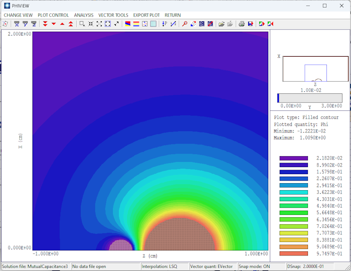
To minimize run time, the calculations were carried out in the first quadrant of the x-y plane, using the natural symmetry conditions of HiPhi at x = 0 and y = 0. Field energy values were multiplied by 4.0 to derive the total capacitances. In the solution, the small sphere is designated as region 1, the large sphere as region 2 and the grounded boundary as region 0. The field energy method, described in Chap. 12 of the HiPhi manual involves making three solutions with a 1.0 V voltage : 1) applied to the small sphere, 2) applied to the large sphere and 3) applied to both spheres. The calculations yield values of the total field energy U1, U2 and U12. Following the derivation in the manual, the capacitances are given by:
C12 = U1 + U2 - U12
C10 = U1 - U2 + U12
C20 = -U1 + U2 + U12
where C12 is the capacitance between the spheres, C10 is the capacitance between the small sphere and the boundary and C20 is the capacitance between the large sphere and the boundary.
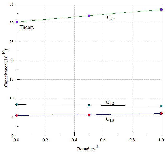
For a solution in a box of width 6.0 cm on a side, the values exhibited significant differences from theory. Assuming that the discrepancies resulted from the finite boundary effect, another solution was performed in a box with side width 12.0 cm. The graph below shows the calculated and theoretical results plotted as a function of the inverse of the boundary width. In this case, infinity corresponds to zero. The projections of the results follow straight lines and agree closely with theory.
|
|
Comments
|
The example illustrates that it takes some work to compare finite-element results (in a limited volume) to ideal benchmarks that involve infinity. On balance, one seldom encounters infinity in real world calculations, and numerical methods are essential for complex electrode shapes and multiple dielectrics. To make comparisons, the geometry was based on a Comsol example.
|