|
Input files
|
Deflector.MIN, Deflector.EIN, Deflector.RIN
Download BeamDeflect.zip
|
|
Description
|
The goal is to generate an approximately uniform transverse electric field inside a cylindrical vacuum chamber to steer a charged-particle beam. Assume an azimuthal array of N rods at radius R that can be biased to different potentials. The question: what are the applied potentials to achieve the best field uniformity? If the goal is an electric field Ey0, then the potential difference at a position x should equal the electric field times the distance along y between electrodes, dV0 = 2*Ey0*R*cos(Theta), where Theta is the angular position of the electrode relative to the y-axis. The potential of electrode N at ThetaN is:
V(N) = Ey0*R*cos(ThetaN).
The result is similar to the Cos(Theta) variation of coil positions to generate a uniform magnetic field inside a circular volume. The demo example geometry has 10 rods with radius 0.4 cm arrayed at a radius of 4.0 cm inside a pipe of radius 5.0 cm. A maximum potential difference of +-1.0 V is applied to the electrodes x = 0.0 cm.
|
|
Results
|
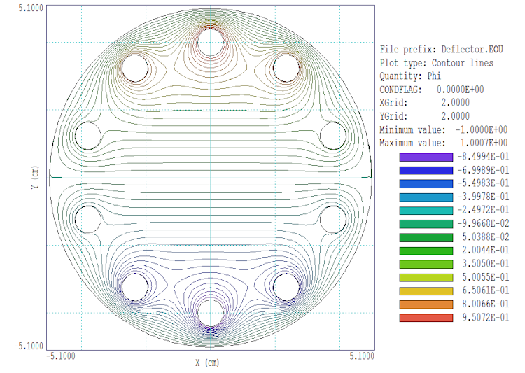
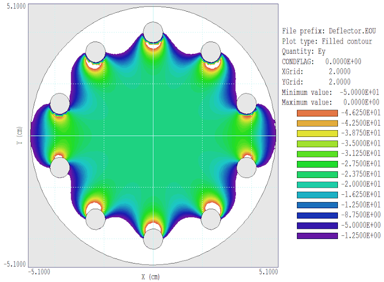
The first step was a calculation with EStat with a variation of voltage magnitude applied to the rods. The predicted electric field with an infinite number of electrodes is Ey0 = 50.0 V/m. The observed field is Ey0(0,0) = 22.74 V/m. The equipotential plot in the top figure shows the reason for the difference. There are significant potential drops between the finite-radius rods and the uniform field region. The secong figure is a color-coded plot of |Ey| with limits set to emphasize field uniformity in the beam volume.
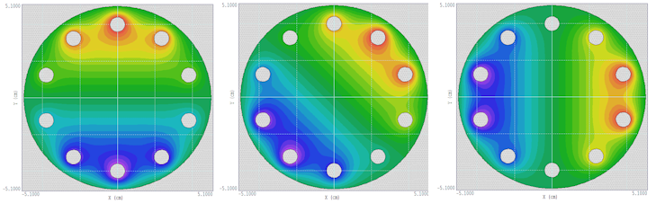
In the second calculation, RFE2 is used to generated a uniform electric field region that rotates at an AC frequency. A potential application is a beam switch that deposits energy over a large-area collector. If we apply harmonic potentials at frequency f with amplitude 1.0 V that vary in phase by 360/N = 36 deg, the potential distribution rotates and is matches the EStat calculation at times separated by interval 1/(N*f). The third figure shows the potential distribution at phases 0.0, 45.0 and 90.0 deg.
|
|
Comments
|
The example illustrates the treatment of ferromagnetic mateials in PerMag and field scaling in the Track mode of Trak.
|