|
Input files
|
PlaneWave.MIN, PlaneWave.WIN, DielectricBoundary.WIN, QuarterWave.WIN
Download PlaneWaves.zip
|
|
Description
|
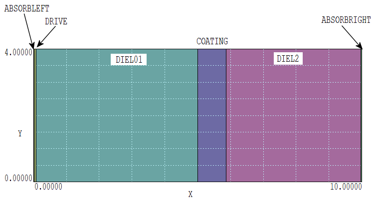
Benchmark WaveSim calculations of electromagnetic wave propagation in unbounded space. Figure 1 shows the geometry. An electromagnetic wave at frequency 7.494 GHz with field components Ey and Hz moves in the x-direction across over a 10 cm distance. The vacuum wavelength is 4.0 cm. Four cases were modeled: 1) uniform vacuum with an absorbing downstream boundary, 2) a reflecting boundary, 3) an absorbing boundary with a transition to a dielectric with EpsiR = 3.0 at 5.0 cm and 4) a transition to the dielectric through a quarter wave layer (thickness 0.8725 cm, EpsiR = 1.732). The examples demonstrate how to generate a travelling wave and how to determine the ratio of standing to traveling waves. |
|
Results
|
Absorbing layers of thickness 0.025 cm are defined at the entrance and exit boundaries. A source of thickness 0.050 cm, adjacent to the entrance absorber, carries a current density at zero phase with magnitude |jy| = 1000 A/m2. The source generates waves moving in the positive and negative directions with theoretical amplitude |Hz| = 1000.0*0.05/2.0 = 0.2500 A/m. The theoretical electric field amplitude is |Ey| = Eta0*Hz0 = 377.0*Ho = 94.25 V/m.
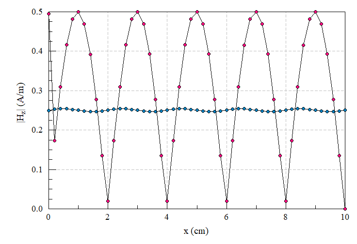
- Case 1, uniform medium with absorbing boundary. WaveSim determines the set of field quantities in phasor notation. Ideally, the amplitudes |Hz| and |Ey| of the propagating wave should be invariant with position. Therefore, a plot of the amplitudes versus x is a sensitive indicator of a standing wave created by a backward traveling wave. The blue symbols of Figure 2 show |Hz| as a function of x. The average value of |Hz| is 0.2498 A/m (within 0.08 of the theoretical prediction) and the average value of |Ey| = 94.56 V/m. The amplitude of the oscillations implies a back traveling wave with amplitude |Hz| = 0.0034 A/m. The reflected wave power density is only 0.018% of the incident wave power. The terminating layer is quite efficient, absorbing 99.98% of the incident wave power.
- Case 2, uniform medium with reflecting boundary. In this case, there are equal forward and backward waves creating a pure standing wave pattern (red symbols of Fig. 1). A wave launched at the upstream source travels forward and backward and terminates in the entrance absorber. Interference between the components creates a standard wave that varies between zero and twice the single wave amplitude, |Hz|max = 0.5 A/m.
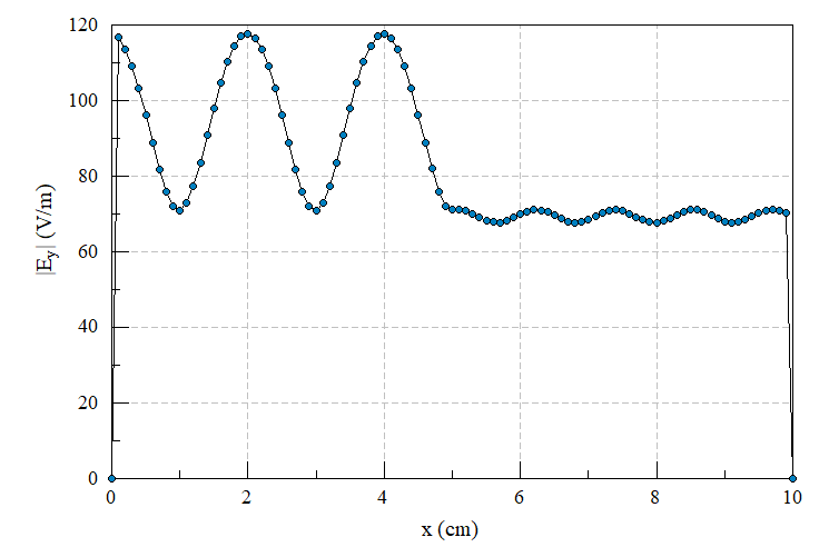
- Case 3, absorbing boundary with a transition to a dielectric with EpsiR = 3.0 at x = 5.0 cm. The dielectric constants are n1 = 1.0 and n2 = sqrt(3) = 1.732. The equations for the reflected and transmitted electric field amplitudes of the waves are Er/Ei = (n1 - n2)/(n1 + n2) = -0.2679 and Et/Ei = 2*n1/(n1 + n2) = 0.732. With Ei = 94.25 V/m, the predicted values are Et = 69.00 V/m and Er = -25.25 V/m. The standing wave in the region x < 5.0 cm should vary between 119.5 V/m and 69.0 V/m. Figure 3 plots the code calculation of |Ey| as a function of x. As expected, there is a standing wave pattern with amplitudes close to the prediction and a pure traveling wave in the dielectric with average amplitude 69.0V/m.
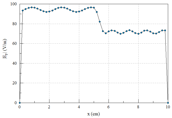
- Case 4, transition from vacuum to the dielectric through a matching quarter wave layer. In this case, n1 = 1.000 and n3 = 1.732. The quarter wave region should have dielectric constant n2 = sqrt(N1*n2) = 1.316. A 7.494 GHz wave in the layer has wavelength (2.998E8)/(7.494E9*1.316) = 3.040 cm. Therefore, the quarter wave layer should have a thickness of 0.7600 cm with EpsiR = 1.732. Figure 4 shows the resulting plot of |Ey|, consistent with pure traveling waves ini both regions, close to the expected amplitudes.
|