I received a package of information from Miki Shen at Magnequench, a manufacturer of neodymium powders for bonded magnets. The E-mailing to developers of magnetic-field software included comprehensive measurements of the properties of their materials. The package represented good marketing and good science. It's surprising how difficult it is to get quality data on magnetic materials.
In this article, I will a explain a bit about what the data mean and show how to integrate them into PerMag and Magnum. The package contained 36 Excel spreadsheets (accessible from OpenOffice) for nine materials at 4 temperatures. Each sheet had a listing and graph of the demagnetization curve in SI and CGS units.
For work with PerMag and Magnum, the SI columns H and B are of interest. The quantity H is the applied magnetic field and B is the total flux density in the material. For the best display of the physics, I prefer to convert H to the applied flux density Bo, where Bo = μoH. If H is expressed in kA-m, the conversion factor to Bo in tesla is 0.0012566. Figure 1 shows a plot of the data for Material MQP-B at 23 ?C. With no applied flux density (Bo = 0), the material has its intrinsic magnetization with a remanance flux density Br = 0.695 tesla. The value is lower than that of a pure neodymium material (1.0-1.2 tesla) because of the bonding filler. Suppose we applied a flux density Bo in the direction opposite that of the magnet. If the material were unaffected, the material and applied flux densities would sum. In this case, the demagnetization curve would be a straight line with slope -1.0 (the green line in the graph). The deviation from the ideal curve indicates the degree of demagnetization of the material. Note that the range of Bo in the graph is broad, extending to the condition of total demagnetization. This information is useful to the manufacturer but is not critical to the designer of a magnet assembly. Clearly, strong demagnetization of materials could not be tolerated in a practical application. The section of the curve near Bo = 0.0 covers most calculations.
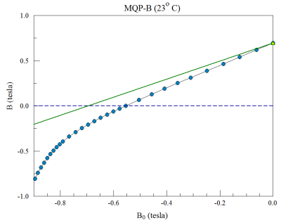
Figure 1. Demagnetization curve example.
Although PerMag could represent the entire nonlinear demagnetization curve, for most applications it is sufficient to use the straight-line approximation for moderate values of Bo. The command to define such a material is
PERMAG RegNo Br Bc Theta
where RegNo is the number of the region representing the magnet, Br is the remanence flux, Bc is the value of Bo where B = 0.0 and θ gives the direction of magnetization (relative to the x or z axis). For the graph below, Br = 0.695 tesla and Bc = -0.550 tesla. The Magnum command is
PERMAG RegNo Br Ux Uy Uz
where Br is the remanence flux and [Ux,Uy,Uz] is a unit vector defining the magnetization direction in three-dimensional space. The assumption in Magnum is that the curve lies close to the ideal straight line. In practice, this approximation introduces only a small error. Here's a link if you would like to download the Magnequench data package: magnequench.zip
LINKS
